Digital Audio Representation
Sound is produced by the rapid backwards and forwards movement of a speaker cone, which disturbs the air. The faster the speaker cone moves, the higher the pitch of sound that is produced.
The speaker cone is moved by an electrically operated magnet (an electromagnet) in response to an applied voltage. In a speaker, the electromagnet is often called the voice coil. Conventionally, a positive voltage moves the speaker cone outwards and a negative voltage moves it inwards. The greater the voltage applied, the louder the sound.

A microphone works like a speaker but the opposite way around. The disturbance of the air caused by someone speaking induces a slight movement in the cone, which is transferred mechanically to the electromagnet. When an electromagnet moves, it produces a voltage in direct proportion to how the cone was moved.
A microphone can be connected to a speaker to produce a telephone. The voltage output from the microphone is transferred to the speaker to produce an exactly corresponding motion in the air somewhere else. The only problem is the signal from the microphone is usually too weak to directly drive a speaker and so we additionally need an amplifier circuit to solve this.
Sound is recorded by taking a continuous measurement of the electrical signal coming from a microphone, which is equivalent to a measurement of exactly how the cone is moving in response to the disturbance of the air. This is often represented on a chart like this as a waveform:
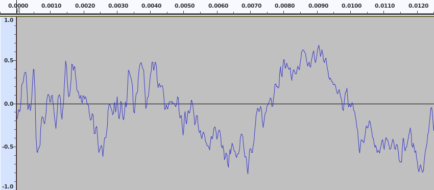
The x-axis of the chart represents time. This section of the waveform represents a very small amount of time, only 0.012 seconds of sound. The y-axis represents the voltage level from the microphone and hence the position of the cone at each specific time measure on the x-axis. When the line is above the centre point, the cone was moving outwards and when the line is below the centre point then the cone was moving inwards.
Sound can be recorded within a physical medium. A (mono) vinyl record stores the waveform by varying the lateral position of a groove in the plastic of the record surface in correspondence to the speaker cone position. The more the groove shifts to one side, the more the speaker cone moves. A cassette tape stores the waveform in the strength of a magnetic field on the tape. This is analogue audio recording.
The problem with analogue recordings is that they degrade over time; the groove in a record wears out and the magnetic field on a tape fades. Imperfections also exist in the copying process and a copy of an analogue recording is never quite the same as the original. The more an analogue recording is copied, the more it deviates from the original recording and the worse the quality.
An alternative approach is we can store the waveform as a table of numbers. We can take readings from the chart and write them down as below. The process of converting the position of the speaker cone at any given time into numbers is known as digitising audio. When we have the sound as a table, we can save it to a file and store it within a computer. Indeed, storage of audio in a computer in this way was originally sometimes known as "wave table" audio, although this term is now less commonly used.
| Time (s) | Cone Position |
|---|---|
| 0.0000 | -0.2 |
| 0.0010 | 0.10 |
| 0.0020 | 0.00 |
| 0.0030 | 0.05 |
| 0.0040 | 0.50 |
| 0.0050 | -0.10 |
| 0.0060 | -0.30 |
| 0.0070 | -0.10 |
| 0.0080 | 0.50 |
| 0.0090 | 0.70 |
| 0.0100 | 0.00 |
| 0.0110 | -0.40 |
| 0.0120 | -0.80 |
We can copy the table of number precisely as many times as we like and it will always be the same table of numbers (provided we verify no mistake was made when copying). The table of numbers will also not fade or change as the medium ages. It will remain the same until the storage device ultimately fails. This is the advantage of digital recording over analogue.
We have taken readings from the chart at intervals of one reading for every 0.0010 seconds. The interval at which we take readings on the time axis is known as the sample rate. On y-axis we have chosen to take readings to a precision of two decimal places. The number of decimal places we choose on the y-axis is the sound resolution.
We can take the table of numbers and plot it to get the waveform back. It looks like this:
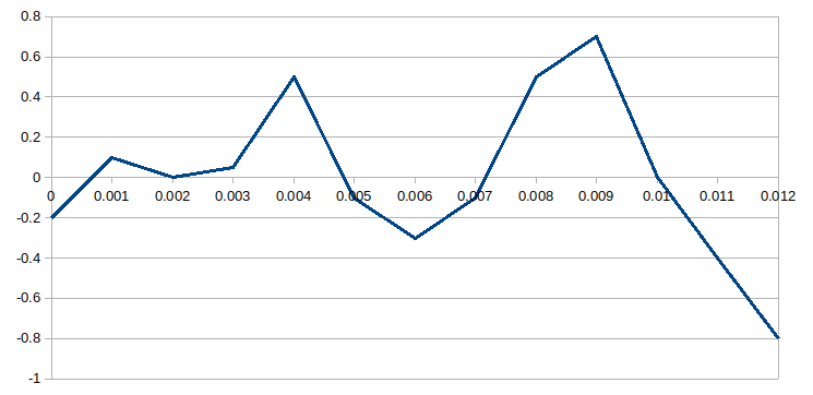
The waveform produced from the table looks somewhat like the original waveform, but it's a long way from a perfect representation. The problem with having a representation that does not very closely match the original waveform is that poor quality audio will result. To solve this problem we can increase the sample rate such that we take measurements from the waveform on the x-axis much more frequently. We can also increase the resolution on the y-axis such that we have more decimal places. Eventually when the sample rate and the resolution are high enough, the reproduction of the waveform from the table of numbers will closely match the original waveform.
Where above we only took a reading every hundredth of a second (one hundred times per second), it is generally agreed that readings, or samples as they are known, need to be taken 44,100 times per second in order to fool the human ear into believing the original waveform is being heard. Resolution on the y-axis is usually expressed in binary bits and 16-bit is normally considered sufficient, that is there are 65,536 discrete positions that the speaker cone can have. This sample rate and resolution is used by compact discs. This was the first digital audio format widely distributed to the public (although not the first digital recording system). The standard has generally stuck and is still used by modern computers and other equipment by default for most general purposes. Other sample rates and resolutions are however in use by professionals and audio enthusiasts.
The popular "WAV" audio file format is just a table of numbers similar to the above representing the position of the speaker cone. The problem with WAV files is they tend to be quite large due to the number of samples that need to be taken to deliver acceptable audio. Clever mathematical techniques have emerged though that can reduce the size of audio files and this is known as data compression. The majority of audio delivered over the internet is compressed.
Image Credits: Luxman audio amplifier, by Wikisympathisant, Creative Commons Attribution-Share Alike 4.0 International license; Speaker image, by Mister rf, Creative Commons Attribution-Share Alike 4.0 International